1.介绍

ggsci 提供一系列高质量的调色板，其灵感来自于科学期刊、数据可视化图书馆、科幻电影和电视节目中使用的颜色。.The color palettes in ggsci are available as ggplot2 scales. For all the color palettes, the corresponding scales are named as:

scale_color_palname()
scale_fill_palname()

We also provided aliases, such as scale_colour_palname() for scale_color_palname().

ggsci所有可用的调色板下表

Name	Scales	Palette Types	Palette Generator
NPG	`scale_color_npg()` `scale_fill_npg()`	`"nrc"`	`pal_npg()`
AAAS	`scale_color_aaas()` `scale_fill_aaas()`	`"default"`	`pal_aaas()`
NEJM	`scale_color_nejm()` `scale_fill_nejm()`	`"default"`	`pal_nejm()`
Lancet	`scale_color_lancet()` `scale_fill_lancet()`	`"lanonc"`	`pal_lancet()`
JAMA	`scale_color_jama()` `scale_fill_jama()`	`"default"`	`pal_jama()`
JCO	`scale_color_jco()` `scale_fill_jco()`	`"default"`	`pal_jco()`
UCSCGB	`scale_color_ucscgb()` `scale_fill_ucscgb()`	`"default"`	`pal_ucscgb()`
D3	`scale_color_d3()` `scale_fill_d3()`	`"category10"` `"category20"` `"category20b"` `"category20c"`	`pal_d3()`
LocusZoom	`scale_color_locuszoom()` `scale_fill_locuszoom()`	`"default"`	`pal_locuszoom()`
IGV	`scale_color_igv()` `scale_fill_igv()`	`"default"` `"alternating"`	`pal_igv()`
UChicago	`scale_color_uchicago()` `scale_fill_uchicago()`	`"default"` `"light"` `"dark"`	`pal_uchicago()`
Star Trek	`scale_color_startrek()` `scale_fill_startrek()`	`"uniform"`	`pal_startrek()`
Tron Legacy	`scale_color_tron()` `scale_fill_tron()`	`"legacy"`	`pal_tron()`
Futurama	`scale_color_futurama()` `scale_fill_futurama()`	`"planetexpress"`	`pal_futurama()`
Rick and Morty	`scale_color_rickandmorty()` `scale_fill_rickandmorty()`	`"schwifty"`	`pal_rickandmorty()`
The Simpsons	`scale_color_simpsons()` `scale_fill_simpsons()`	`"springfield"`	`pal_simpsons()`
GSEA	`scale_color_gsea()` `scale_fill_gsea()`	`"default"`	`pal_gsea()`
Material Design	`scale_color_material()` `scale_fill_material()`	`"red"` `"pink"` `"purple"` `"deep-purple"` `"indigo"` `"blue"` `"light-blue"` `"cyan"` `"teal"` `"green"` `"light-green"` `"lime"` `"yellow"` `"amber"` `"orange"` `"deep-orange"` `"brown"` `"grey"` `"blue-grey"`	`pal_material()`

2 Discrete Color Palettes

We will use scatterplots with smooth curves, and bar plots to demonstrate the discrete color palettes in ggsci.

library("ggsci")
library("ggplot2")
library("gridExtra")

data("diamonds")

p1 = ggplot(subset(diamonds, carat >= 2.2),
       aes(x = table, y = price, colour = cut)) +
  geom_point(alpha = 0.7) +
  geom_smooth(method = "loess", alpha = 0.05, size = 1, span = 1) +
  theme_bw()

p2 = ggplot(subset(diamonds, carat > 2.2 & depth > 55 & depth < 70),
       aes(x = depth, fill = cut)) +
  geom_histogram(colour = "black", binwidth = 1, position = "dodge") +
  theme_bw()

2.1 NPG

The NPG palette is inspired by the plots in the journals published by Nature Publishing Group:

p1_npg = p1 + scale_color_npg()
p2_npg = p2 + scale_fill_npg()
grid.arrange(p1_npg, p2_npg, ncol = 2)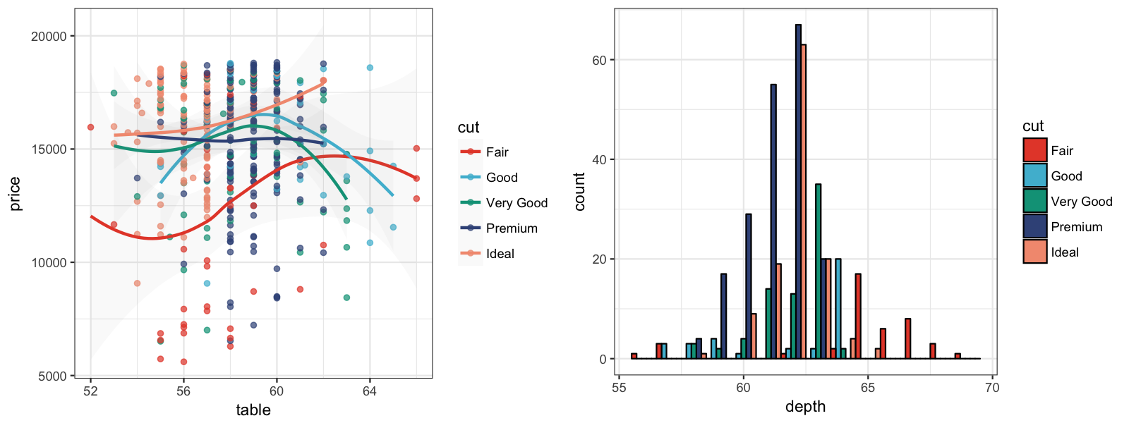

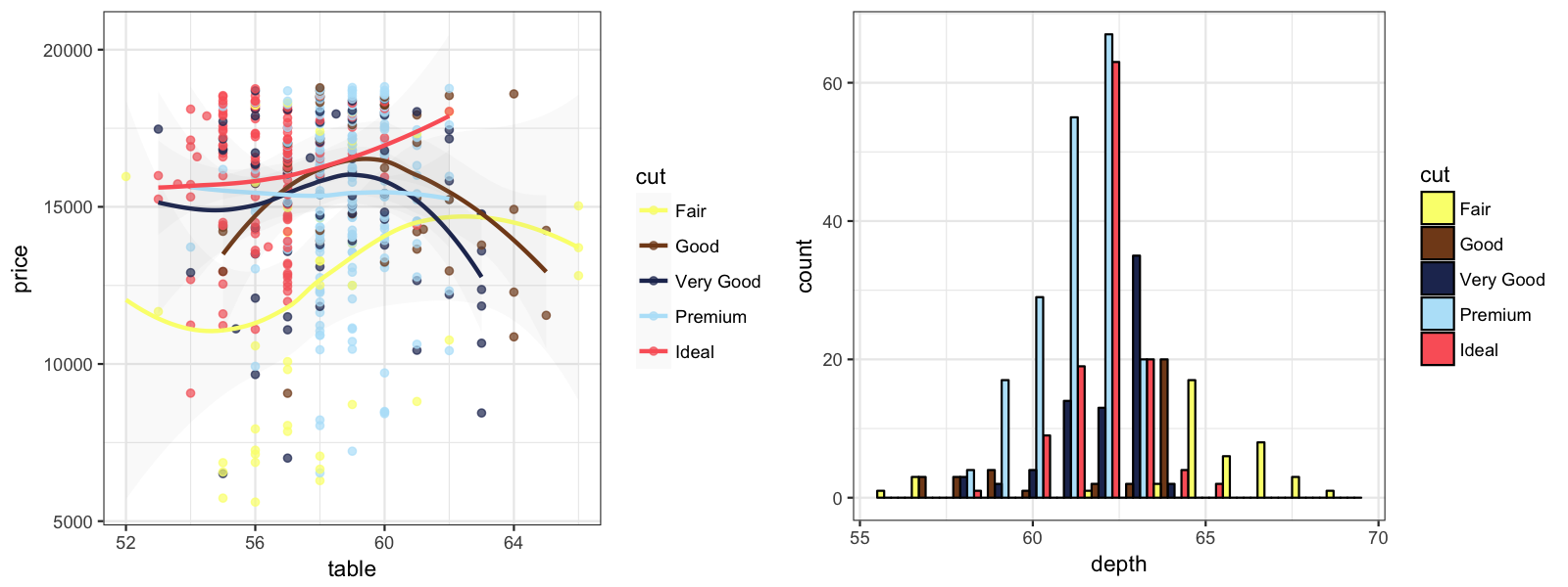
2.2 AAAS

The AAAS palette is inspired by the plots in the journals published by American Association for the Advancement of Science:

p1_aaas = p1 + scale_color_aaas()
p2_aaas = p2 + scale_fill_aaas()
grid.arrange(p1_aaas, p2_aaas, ncol = 2)

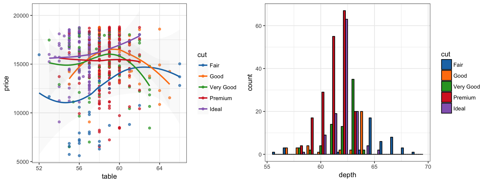
2.3 NEJM

The NEJM palette is inspired by the plots in The New England Journal of Medicine:

p1_nejm = p1 + scale_color_nejm()
p2_nejm = p2 + scale_fill_nejm()
grid.arrange(p1_nejm, p2_nejm, ncol = 2)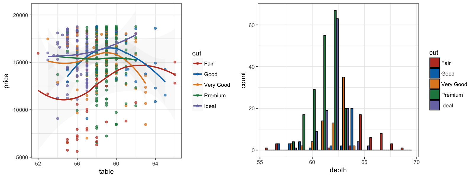

2.4 Lancet

The Lancet palette is inspired by the plots in Lancet journals, such as Lancet Oncology:

p1_lancet = p1 + scale_color_lancet()
p2_lancet = p2 + scale_fill_lancet()
grid.arrange(p1_lancet, p2_lancet, ncol = 2)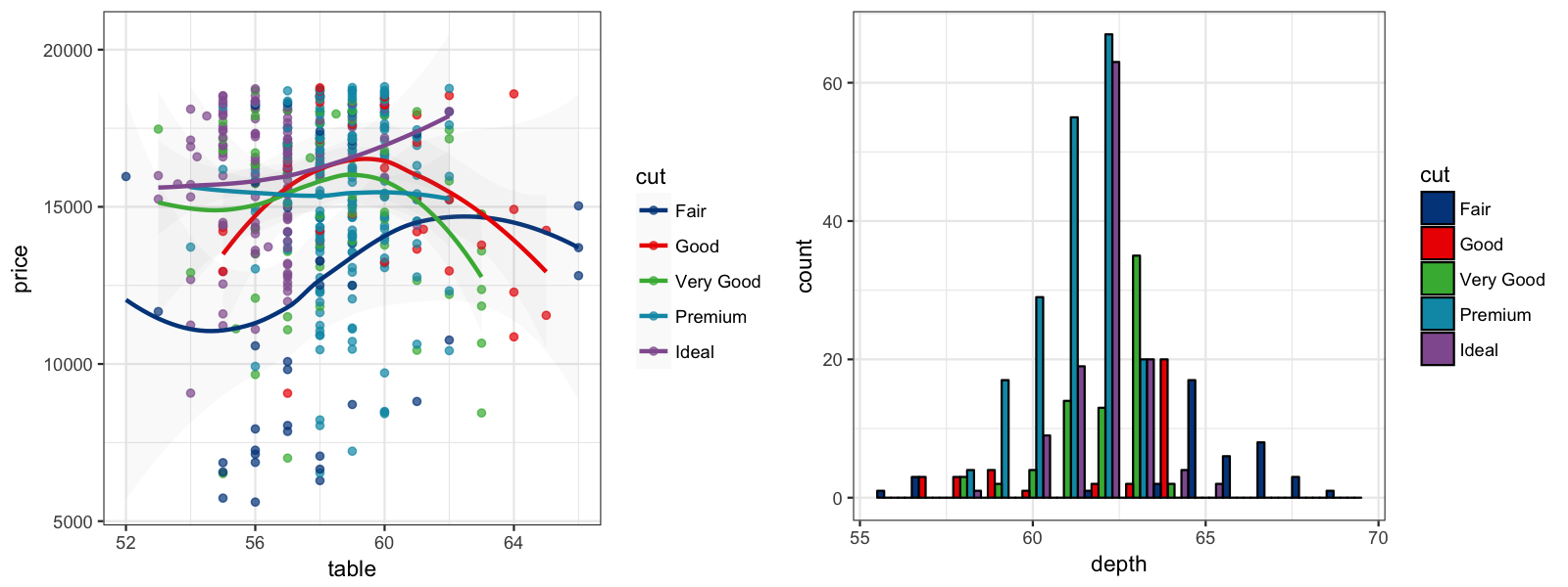

2.5 JAMA

The JAMA palette is inspired by the plots in The Journal of the American Medical Association:

p1_jama = p1 + scale_color_jama()
p2_jama = p2 + scale_fill_jama()
grid.arrange(p1_jama, p2_jama, ncol = 2)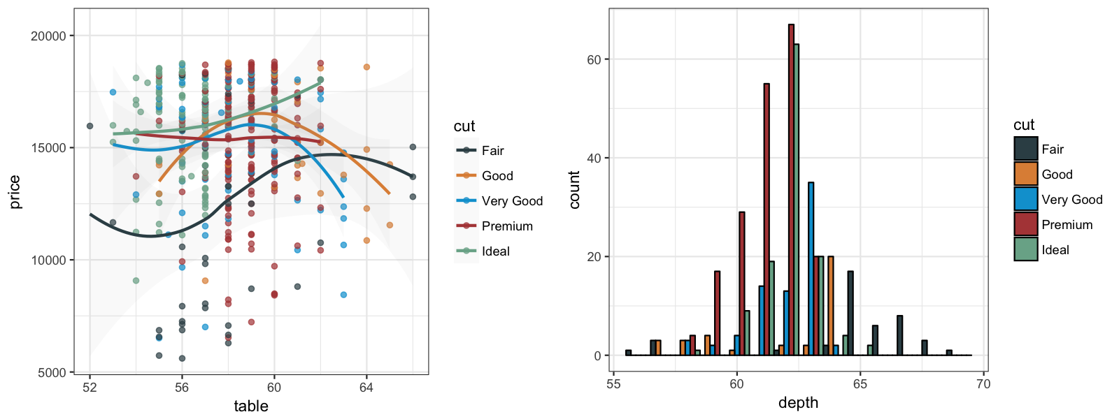

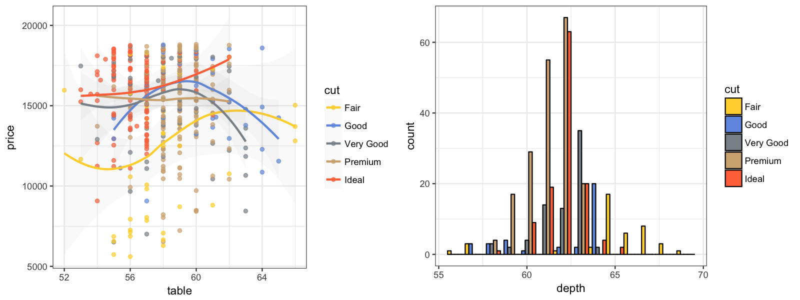
2.6 JCO

The JCO palette is inspired by the the plots in Journal of Clinical Oncology:

p1_jco = p1 + scale_color_jco()
p2_jco = p2 + scale_fill_jco()
grid.arrange(p1_jco, p2_jco, ncol = 2)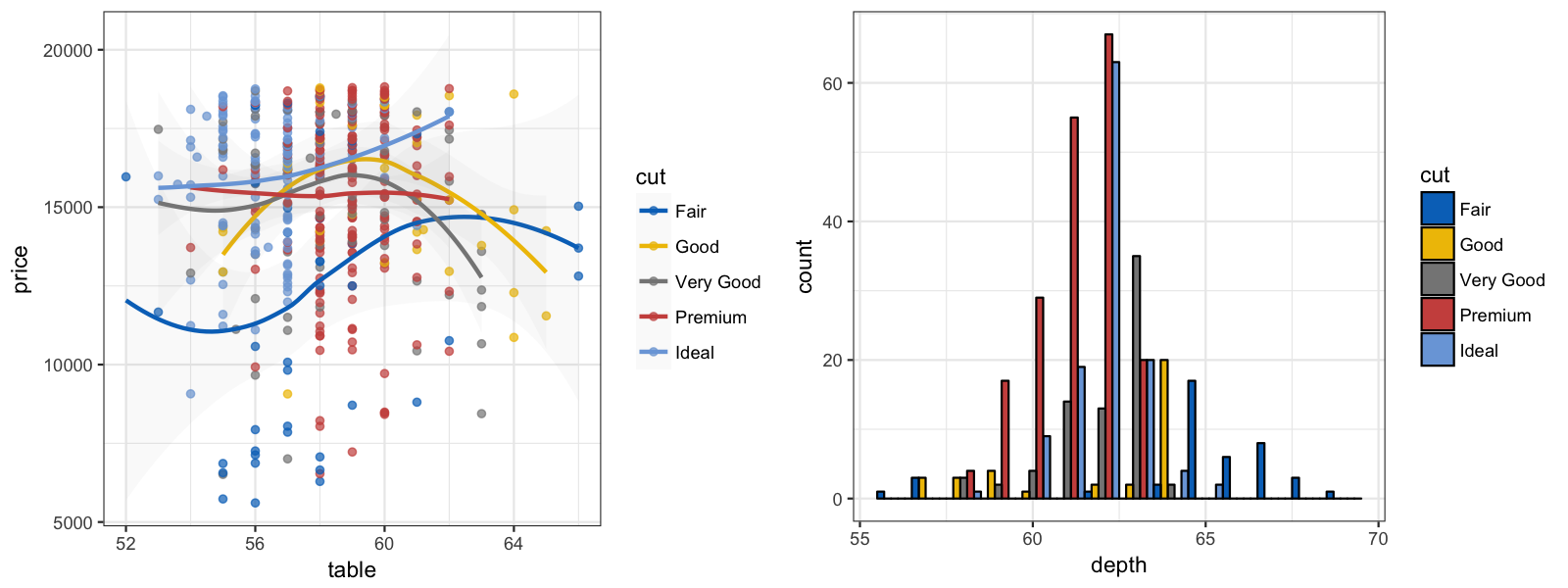

2.7 UCSCGB

The UCSCGB palette is from the colors used by UCSC Genome Browser for representing chromosomes. This palette has been intensively used in visualizations produced by Circos.

p1_ucscgb = p1 + scale_color_ucscgb()
p2_ucscgb = p2 + scale_fill_ucscgb()
grid.arrange(p1_ucscgb, p2_ucscgb, ncol = 2)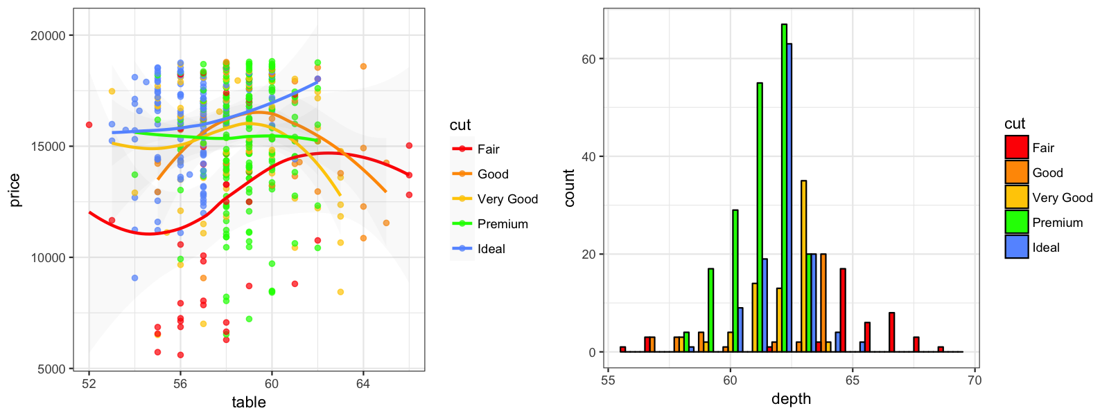

2.8 D3

The D3 palette is from the categorical colors used by D3.js (version 3.x and before). There are four palette types (category10, category20, category20b, category20c) available.

p1_d3 = p1 + scale_color_d3()
p2_d3 = p2 + scale_fill_d3()
grid.arrange(p1_d3, p2_d3, ncol = 2)

2.9 LocusZoom

The LocusZoom palette is based on the colors used by LocusZoom.

p1_locuszoom = p1 + scale_color_locuszoom()
p2_locuszoom = p2 + scale_fill_locuszoom()
grid.arrange(p1_locuszoom, p2_locuszoom, ncol = 2)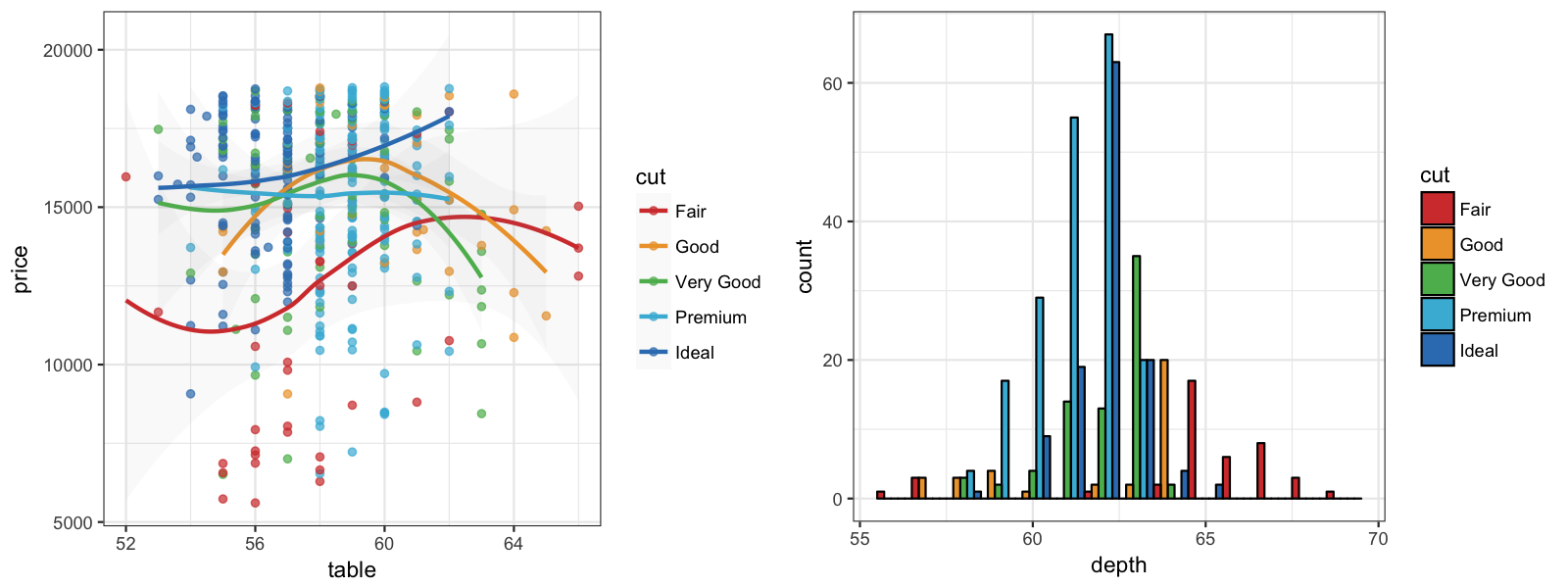

2.10 IGV

The IGV palette is from the colors used by Integrative Genomics Viewer for representing chromosomes. There are two palette types (default, alternating) available.

p1_igv_default = p1 + scale_color_igv()
p2_igv_default = p2 + scale_fill_igv()
grid.arrange(p1_igv_default, p2_igv_default, ncol = 2)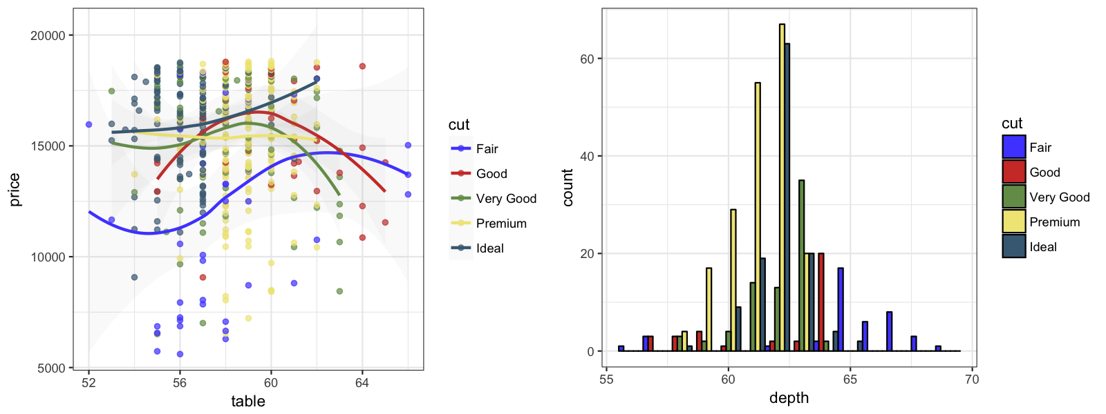

2.11 UChicago

The UChicago palette is based on the colors used by the University of Chicago. There are three palette types (default, light, dark) available.

p1_uchicago = p1 + scale_color_uchicago()
p2_uchicago = p2 + scale_fill_uchicago()
grid.arrange(p1_uchicago, p2_uchicago, ncol = 2)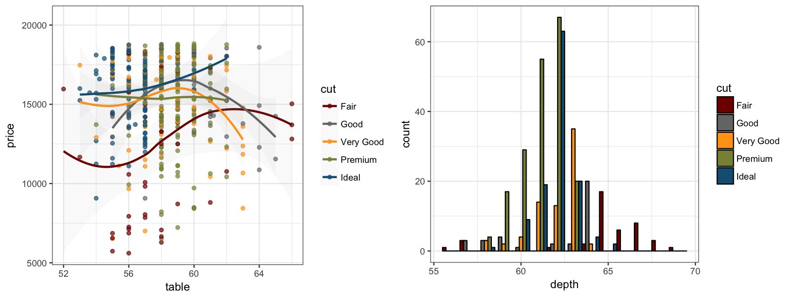

2.12 Star Trek

This palette is inspired by the (uniform) colors in Star Trek:

p1_startrek = p1 + scale_color_startrek()
p2_startrek = p2 + scale_fill_startrek()
grid.arrange(p1_startrek, p2_startrek, ncol = 2)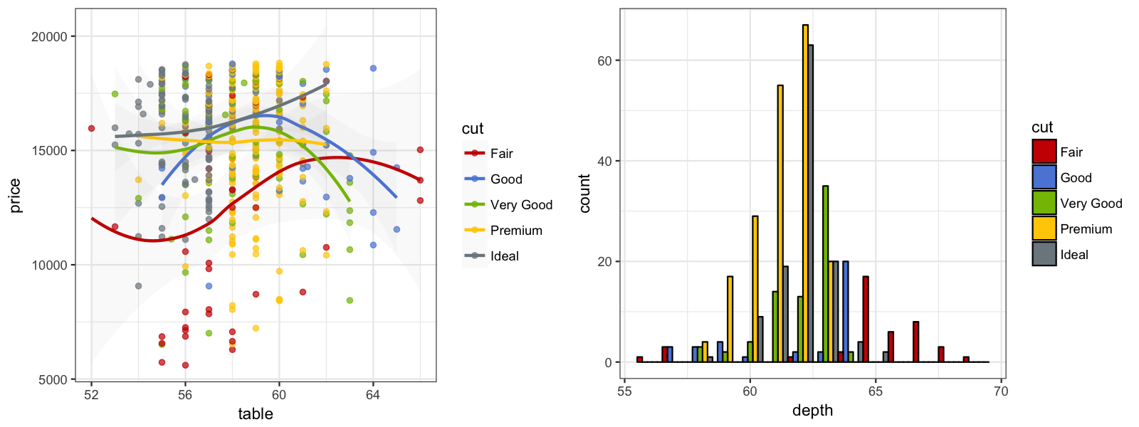

2.13 Tron Legacy

This palette is inspired by the colors used in Tron Legacy. It is suitable for displaying data when using a dark theme:

p1_tron = p1 + theme_dark() + theme(
    panel.background = element_rect(fill = "#2D2D2D"),
    legend.key = element_rect(fill = "#2D2D2D")) +
  scale_color_tron()
p2_tron = p2 + theme_dark() + theme(
    panel.background = element_rect(fill = "#2D2D2D")) +
  scale_fill_tron()
grid.arrange(p1_tron, p2_tron, ncol = 2)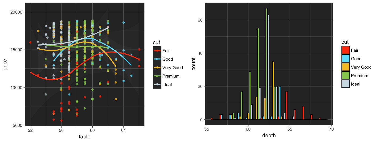

2.14 Futurama

This palette is inspired by the colors used in the TV show Futurama:

p1_futurama = p1 + scale_color_futurama()
p2_futurama = p2 + scale_fill_futurama()
grid.arrange(p1_futurama, p2_futurama, ncol = 2)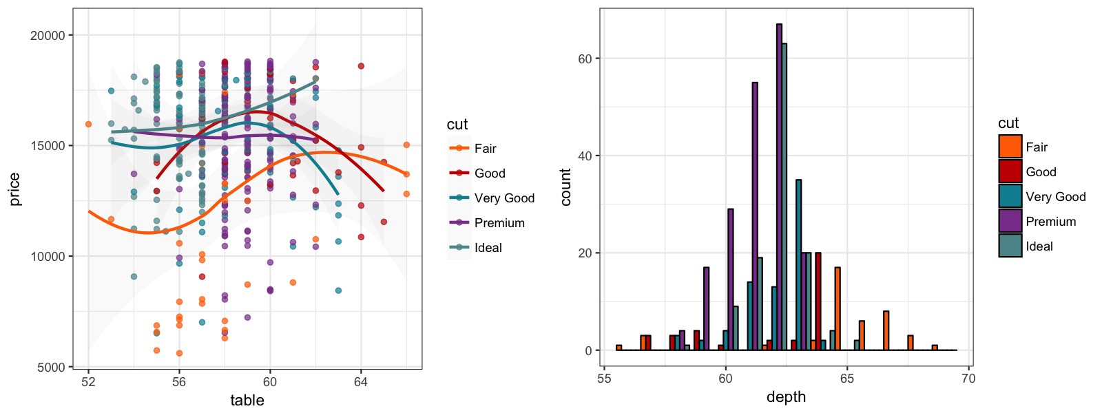

2.15 Rick and Morty

This palette is inspired by the colors used in the TV show Rick and Morty:

p1_rickandmorty = p1 + scale_color_rickandmorty()
p2_rickandmorty = p2 + scale_fill_rickandmorty()
grid.arrange(p1_rickandmorty, p2_rickandmorty, ncol = 2)

2.16 The Simpsons

This palette is inspired by the colors used in the TV show The Simpsons:

p1_simpsons = p1 + scale_color_simpsons()
p2_simpsons = p2 + scale_fill_simpsons()
grid.arrange(p1_simpsons, p2_simpsons, ncol = 2)

3 Continuous Color Palettes

We will use a correlation matrix visualization (a special type of heatmap) to demonstrate the continuous color palettes in ggsci.

library("reshape2")

data("mtcars")
cor = cor(unname(cbind(mtcars, mtcars, mtcars, mtcars)))
cor_melt = melt(cor)

p3 = ggplot(cor_melt,
            aes(x = Var1, y = Var2, fill = value)) +
  geom_tile(colour = "black", size = 0.3) +
  theme_bw() +
  theme(axis.title.x = element_blank(),
        axis.title.y = element_blank())

3.1 GSEA

The GSEA palette (continuous) is inspired by the heatmaps generated by GSEA GenePattern.

p3_gsea     = p3 + scale_fill_gsea()
p3_gsea_inv = p3 + scale_fill_gsea(reverse = TRUE)
grid.arrange(p3_gsea, p3_gsea_inv, ncol = 2)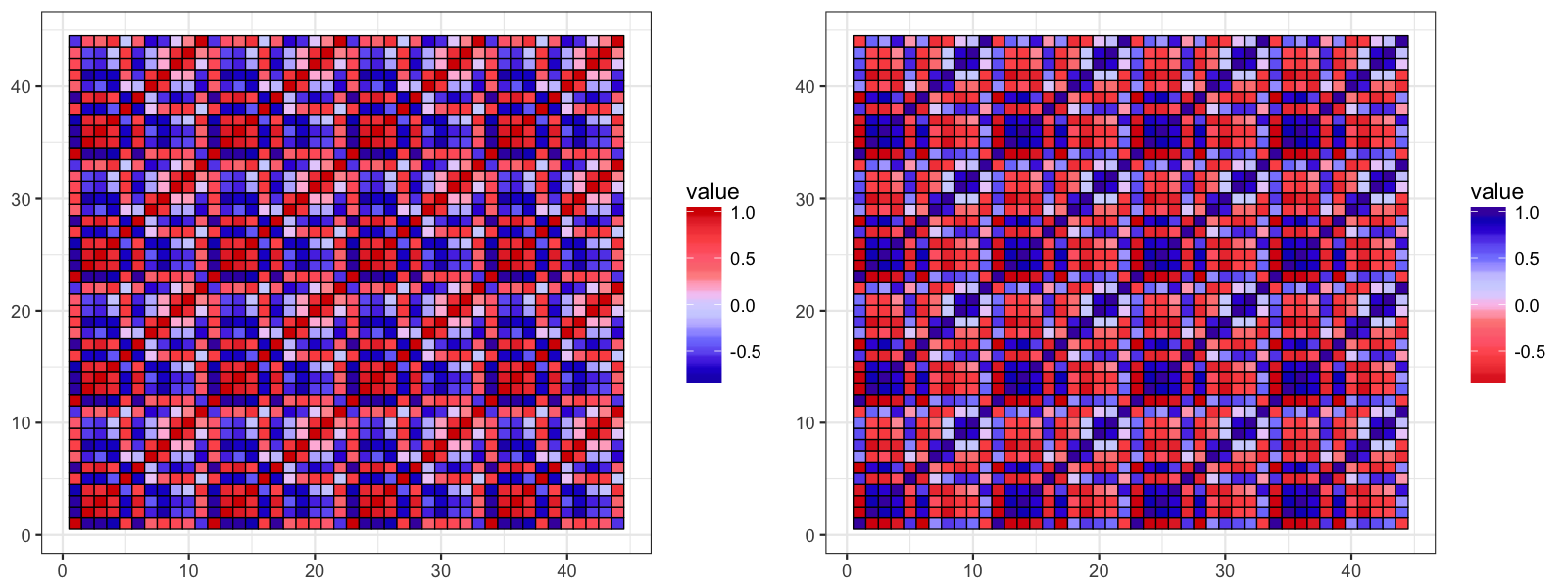

3.2 Material Design

The Material Design color palettes are from the material design color guidelines.

We generate a random matrix first:

library("reshape2")

set.seed(42)
k = 9
x = diag(k)
x[upper.tri(x)] = runif(sum(1:(k - 1)), 0, 1)
x_melt = melt(x)

p4 = ggplot(x_melt, aes(x = Var1, y = Var2, fill = value)) +
  geom_tile(colour = "black", size = 0.3) +
  scale_x_continuous(expand = c(0, 0)) +
  scale_y_continuous(expand = c(0, 0)) +
  theme_bw() + theme(
    legend.position = "none", plot.background = element_blank(),
    axis.line = element_blank(), axis.ticks = element_blank(),
    axis.text.x = element_blank(), axis.text.y = element_blank(),
    axis.title.x = element_blank(), axis.title.y = element_blank(),
    panel.background = element_blank(), panel.border = element_blank(),
    panel.grid.major = element_blank(), panel.grid.minor = element_blank())

Plot the matrix with the 19 material design color palettes:

grid.arrange(
  p4 + scale_fill_material("red"),         p4 + scale_fill_material("pink"),
  p4 + scale_fill_material("purple"),      p4 + scale_fill_material("deep-purple"),
  p4 + scale_fill_material("indigo"),      p4 + scale_fill_material("blue"),
  p4 + scale_fill_material("light-blue"),  p4 + scale_fill_material("cyan"),
  p4 + scale_fill_material("teal"),        p4 + scale_fill_material("green"),
  p4 + scale_fill_material("light-green"), p4 + scale_fill_material("lime"),
  p4 + scale_fill_material("yellow"),      p4 + scale_fill_material("amber"),
  p4 + scale_fill_material("orange"),      p4 + scale_fill_material("deep-orange"),
  p4 + scale_fill_material("brown"),       p4 + scale_fill_material("grey"),
  p4 + scale_fill_material("blue-grey"),
  ncol = 6)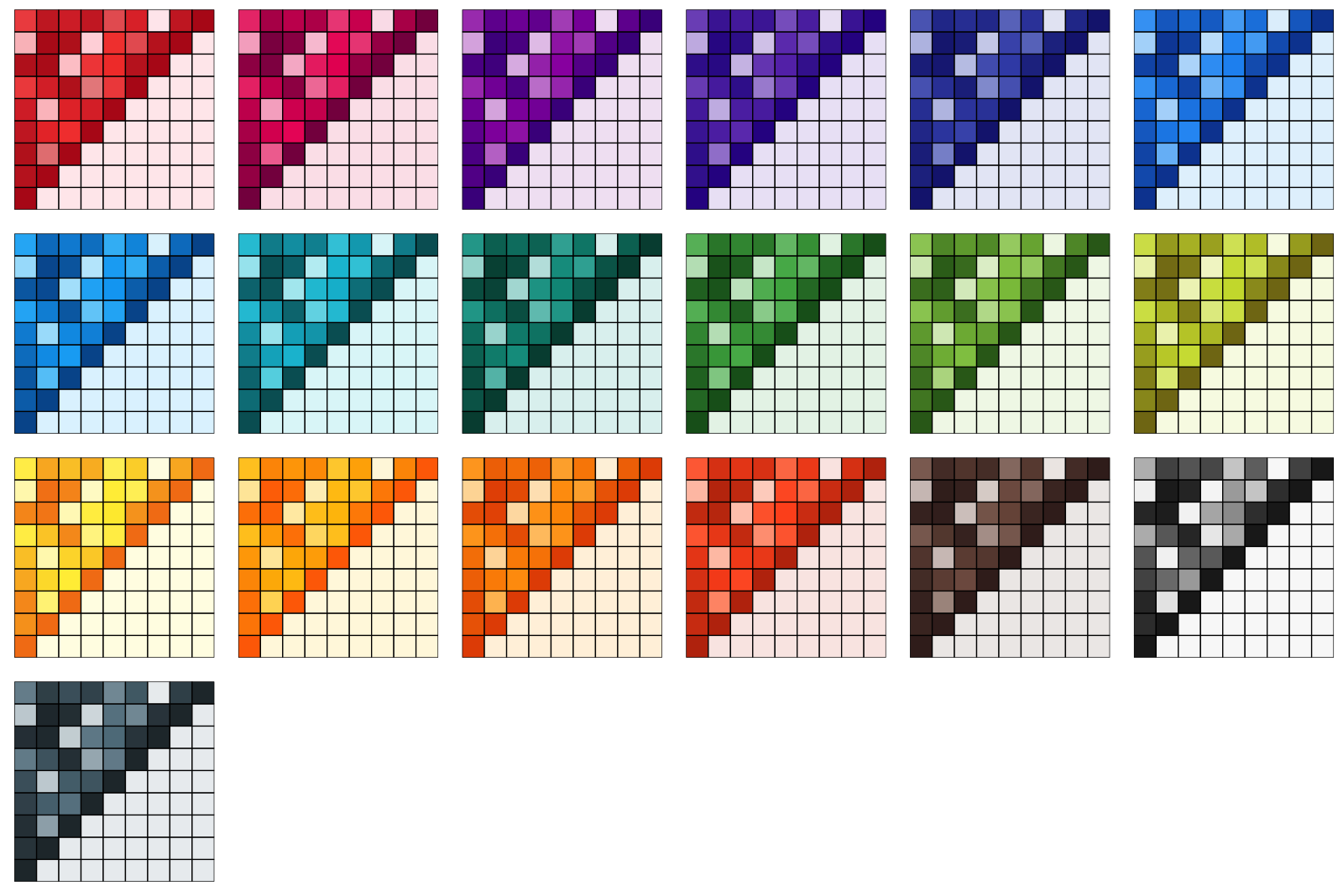

From the figure above, we can see that even though an identical matrix was visualized by all plots, some palettes are more preferrable than the others because our eyes are more sensitive to the changes of their saturation levels.

4 Non-ggplot2 Graphics

To apply the color palettes in ggsci to other graphics systems (such as base graphics and lattice graphics), simply use the palette generator functions in the table above. For example:

mypal = pal_npg("nrc", alpha = 0.7)(9)
mypal

## [1] "#E64B35B2" "#4DBBD5B2" "#00A087B2" "#3C5488B2" "#F39B7FB2" "#8491B4B2"
## [7] "#91D1C2B2" "#DC0000B2" "#7E6148B2"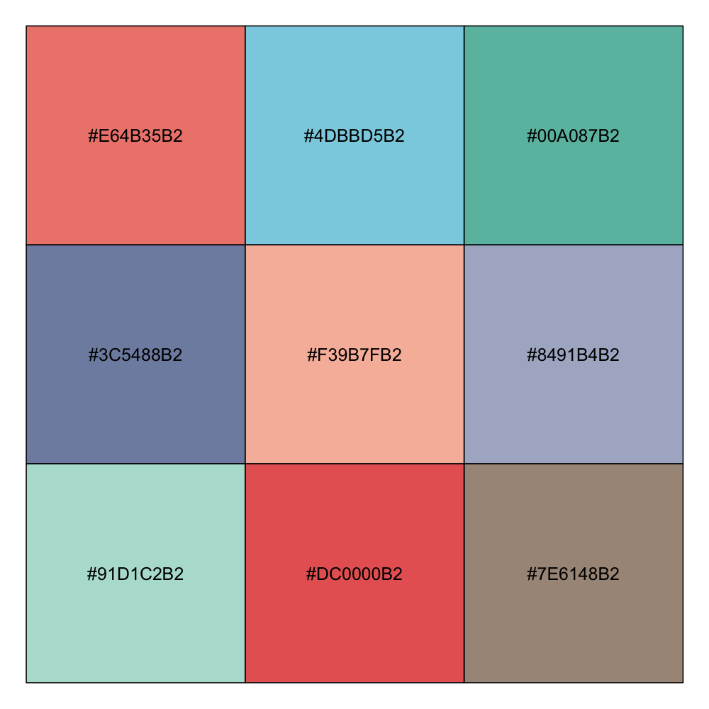

library("scales")
show_col(mypal)

You will be able to use the generated hex color codes for such graphics systems accordingly. The transparent level of the entire palette is easily adjustable via the argument "alpha" in every generator or scale function.

5 Discussion

请注意，有些调色板可能不是某些目的的最佳选择，如色盲安全、复印安全或打印友好。如果你确实有这样的考虑，你可能想看看ColorBrewer和viridis这样的调色板。

如若转载，请注明出处：https://www.ouq.net/1837.html

ggsci:ggplot2科学期刊主题调色板